Table of Contents

1. Flocking Behaviour in Nature
2. The Boids Algorithm
3. The Implementation
   1. Python Implementation
   2. C Implementation

Flocking Behaviour in Nature

One of the definitions of a flock in the Merraim-Webster Dictionary is as follows:

“a group of animals (such as birds or sheep) assembled or herded together”

Flocking is a common self-organizing and self-regulating behaviour among a variety of creatures in nature. From a Dazzle of Zebras migrating across the Savannah to a School of Herrings dancing in the Atlantic, all represent a kind of behaviour that becomes interesting when a bunch of animals, birds, or fish act and interact with each other as a group.

Perhaps, this is best exemplified by the stunning shapes and forms created by a Murmuration of Starlings swaying in the open sky. The behaviour of a single Starling by itself is not that interesting but when a flock of Starlings takes to the sky, it is a sight to behold.

The Boids Algorithm

We will now take a look at an algorithm for describing the flocking behaviour of agents (animals, birds, fish, et cetera). We define an agent as an entity that has a well-defined and monotonous behaviour e.g. an entity that keeps moving straight until it encounters a boundary, at which point, it proceeds toward another direction. We will see how we can simulate seemingly choreographed behaviour of a collection of such agents following three simple rules.

The algorithm is called Boids. It was developed in the 80s by Craig W. Reynolds He created this model to simulate the movement of a flock of birds, hence the name Boids (Bird-oids). Each boid follows the rules specified by the algorithm and as a result, an interesting flocking behaviour emerges.

The rules^[1] are as follows:

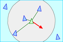
1. Separation: Steer to avoid crowding local flockmates

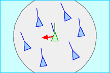
2. Alignment: Steer towards the average heading of local flockmates

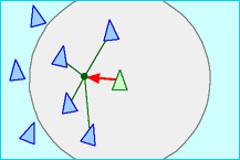
3. Cohesion: Steer to move toward the average position of local flockmates

The circle visible in these illustrations represent the field of view of each boid. It is the effective range (or the neighbourhood) within which the rules apply to the boid. It is determined by parameters, distance and angle i.e. distance from center of the boid (radius) and angle with respect the direction of the boid’s velocity. Here, we will be completely ignoring the angle and suppose that all neighbouring boids within the perimeter of the circle are visible to the boid.

The Implementation

Python Implementation

Implementing the algorithm is a straighforward task. We can use pygame to create the simulation. Each boid object has a position (x, y) and velocity (vx, vy). We spawn a specified number of boids and store them in the flock array. We iterate through the flock array and for each boid, we average the relevant position and velocity values of its neighbouring boids as indicated by the boid’s visual_range. A constant, protected_range is introduced which, when paired together with the avoid_factor parameters keeps the boids spaced such that they don’t collide or overlap, as in our case, we are not doing any actual collision detection.

We then modify the boid position and velocity based on the difference of their current value and the neighbourhood average. A couple of parameters are used here. matching_factor and centering_factor are respectively used to modulate the effect of velocity average and position average on the boid’s velocity, which subsequently affects its position.

Similarly, turning_factor is used to smoothly turn the boid when it reaches the window boundary.

This first attempt, while functional, is extremely inefficient. The way this algorithm is implemented leads to a quadratic time complexity. As a result, simulating even a few hundred boids becomes slow and computationally demanding. The first step towards optimizing the algorithm is realising that it is completely unnecessary to compare each boid with every other boid. Because a boid may only flock with a limited number of boids in its vicinity, the number of comparisons would be greatly reduced if we could figure out a way of accessing only those boids which might possibly be within the visual_range of that boid. We can achieve this by using a special Hash table, called a Spatial Hash Grid.

Optimization: Spatial Hash Grid

A Spatial Hash Grid is a hash table that puts points(x, y) in space into cells in the hash table. Consider each dot on the following illustration to be a boid. The total space is divided into a number of cells and each boid is hashed into a cell.

In this implementation, each boid is a point on the grid, which means that no boid will ever belong to more than one cell on the grid. So, we can further simplify the hashing process and bin each point into its corresponding cell by using the following hash function.

def hash_function(b_x, b_y):
    x = int(b_x / cell_size)
    y = int(b_y / cell_size)
    return x + y * window_cols

Using this Spatial Hash Grid, we can now compare only those boids which lie in the cells in the vicinity of a particular boid. We introduce a new parameter called vicinity here. The vicinity of each boid is represented as a square in the following screenshot. It is necessary for this parameter to be slightly larger than the visual_range of the boid, otherwise, it may exclude potentially neighbouring boids.

Observe that the vicinity overlaps a number of cells starting at its top-left corner and ending at its bottom-right corner. We use this observation to accumulate all potentially neighbouring boids into a set and perform comparisons with those boids. This greatly decreases the complexity of the algorithm and allows us to simulate almost five hundred boids smoothly.

C Implementation

I guarantee that after playing around with the simulation for some time, the urge to have a gazillion boids swirling around the screen will suddenly overcome you. The python implementation, at least in my computer, can only manage 500 simultaneous boids even with the optimization. So, I translated the python code into C line by line and the result was amazing.

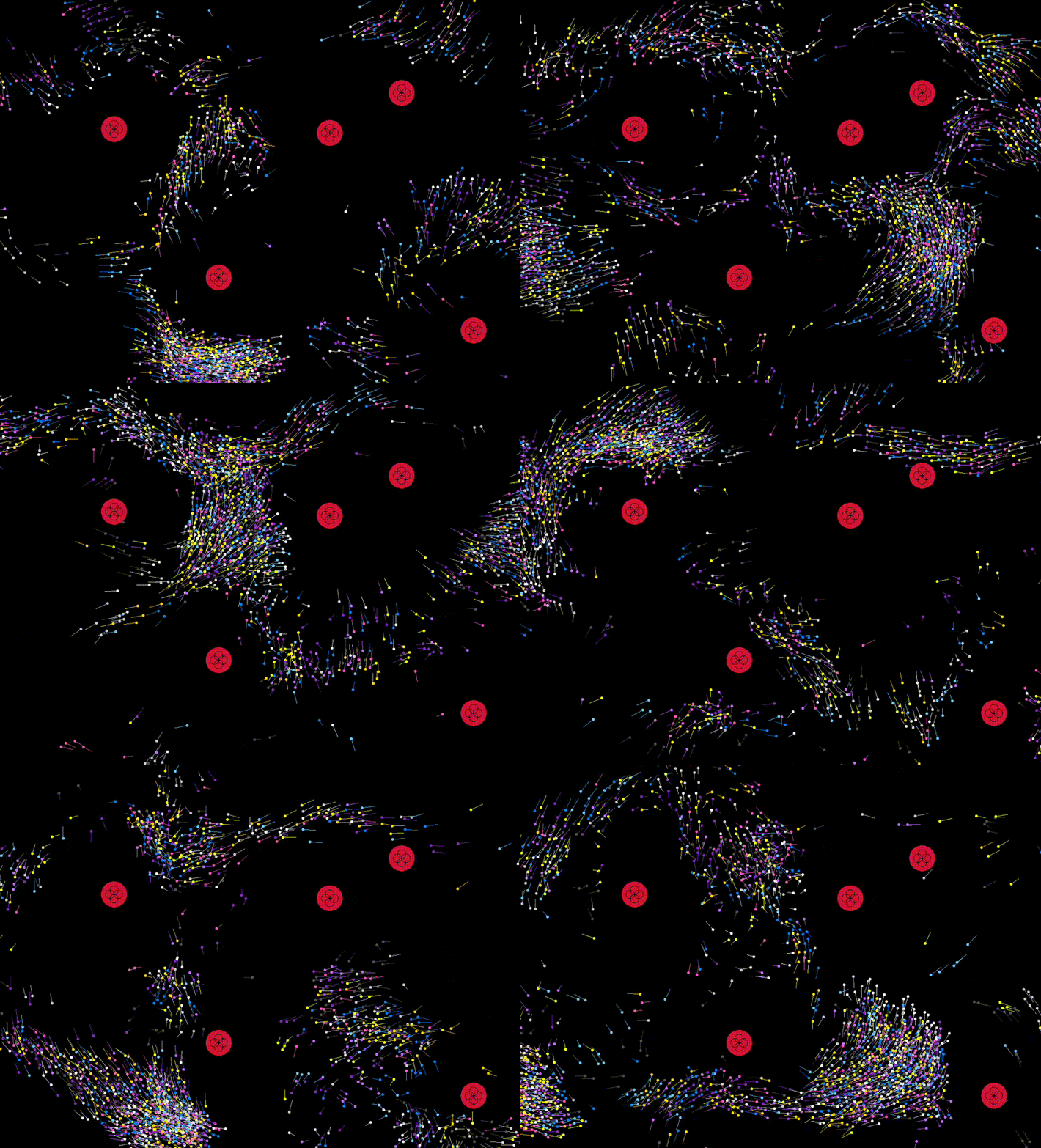
The gif below shows the C implementation comfortably simulating 2000 boids. I have allowed different coloured boids to flock with each other as I figured it would lead to a more interesting result.

I have also introduced an obstacle entity. It is essentially the same as a boid but the only difference is that it remains at one point and alters the velocity of the boids that come close to it away from it based on a obstacle_turn_factor.

The full source code for the C implementation is available here.

If you’re interested in the Python implementation, feel free to reach out to me.

1. These rules and accompanying illustrations are directly borrowed form Craig’s Original Paper. ↩