Published on November 26, 2024

Cellular Automata

9 minutes read •

Table of Contents


                  ████
              ██████████            ██
            ██        ██████  ██      ██████
            ██    ████████          ██      ████
            ████    ██    ██  ██    ██        ██
                ████        ████          ██  ████
                              ████      ██  ████
                                    ██████████
                                ████    ████

What are Cellular Automata and why are they interesting?

Automata is the plural form of automaton. In automata theory, an automaton can be described as a discrete model of computation that has a number of states and has rules for transitioning between those states. Thus, Cellular Automata(CA) are a class of automata that operate over a grid of cells, where each cell can have a finite number of states and transitions between those states based on the state of its neighboring cells. Cellular Automata are discrete, meaning that the cells transition between different states in discrete time-steps. The overall state of the CA at any time-step is called a generation. The history of Cellular Automata goes back to the 40s and their application is mostly in the modeling of various physical, biological or even sociological phenomena.

In the last article, I discussed about the idea of emergence and how even agents with limited capabilities, governed by simple rules, can generate surprisingly complex behaviour. Here, I continue the discussion of emergent behaviour in the context of Cellular Automata. Take the popular two-dimensional Cellular Automaton, Conway’s Game of Life, or Life for short, devised by the British mathematician, John Conway. Like in the case of many CA, the rules for Life are simple and deterministic. Each cell can either be dead or alive. A dead cell in a generation, becomes alive in the next if it has exactly three live neighbors (Moore Neighborhood or N8) by reproduction. A live cell in a generation dies in the next if it has fewer than two live neighbors or more than three live neighbors, respectively by underpopulation and overpopulation. In all other cases, the state of the cell remains the same.

Following these simple deterministic rules, rich and complex behaviour emerges, behaviour that couldn’t be predicted simply by looking at the random combination of dead and alive cells in the starting generation. People have studied the evolution of different patterns in the Life and have discovered intersting behaviour among certain patterns. There are still lifes that are stable configurations that sustain indefinitely, oscillators that transition between a number of configurations in a cyclical manner (the number of configurations is referred to as the period of the oscillator), and spaceships that are like oscillators but travel across the grid, the most popular being the glider that travels diagonally along the grid. Another intersting pattern in the Game of Life is the Gosper Glider Gun. This pattern emits a glider every 30 generations. It is one of the patterns that exhibits infinite growth.

It has been shown that by combining different patterns, logic gates and latches can be constructed in Life. The implication of this is broad, and it means that, theoretically speaking, the Game of Life is capable of performing all computations that the computers we use are capale of. In short, it is Turing Complete. People have made everything from simple adder and subtractor circuits to clocks in Life. Perhaps, the most interesting one is this simulation of Life in Life by Phillip Bradbury. Take a minute to watch the video and contemplate its larger meaning. Fair Warning! I refuse to take responsibility if it evokes a sudden feeling of existential crisis in you.

Some Popular Cellular Automata

Conway’s Game of Life

Here is my implementation of Conway’s Game of Life in python.

Show

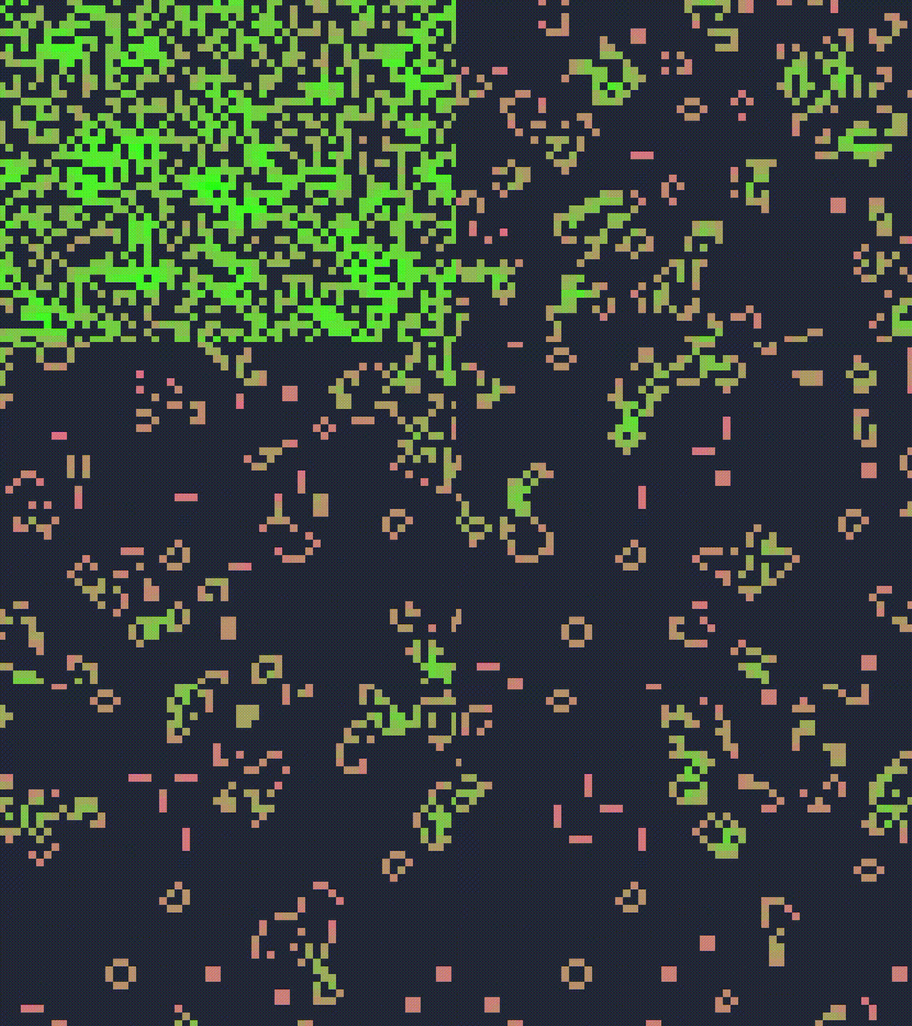
Brian’s Brain

It was invented by Brian Silverman. It is similar to the Game of Life but it adds an extra state. It is supposed to model the state of neurons in the brain, so the three states can be described as:

Off and ready to fire,
Firing (On) and
Refractory after firing (Dying)

The Rules for the CA are written as a python program as follows:

if current_state == 0:
    if (no_of_neighbors == 2):
        return 1
    return 0  # same state
if current_state == 1:
    return 2
if current_state == 2:
    return 0

Here states 0, 1 and 2 respectively correspond to off, on and dying.

Most patterns in Brian’s Brain explode into a chaotic ensemble of spaceships, rakes, breeders and so on that seemingly go on indefinitely. This CA is also Turing Complete.

Show

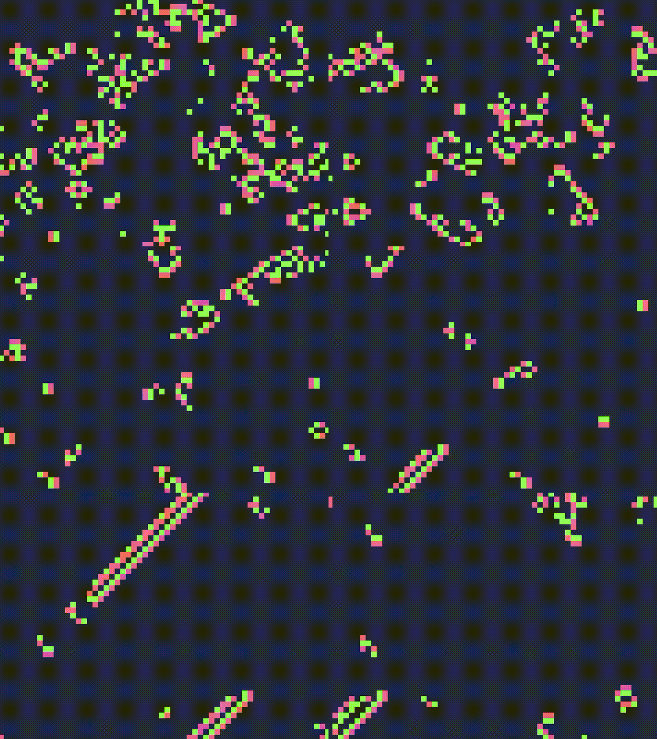
Brain Life

While researching for this article, I came across a manual for an old software called CellLab that was developed in the late 1980s by Rudy Rucker and John Walker. The former being an author of popular sci-fi novels and the latter, of course, one of the co-founders of Autodesk. While the manual was extremely informative in itself, I found it to be a curious piece of history of research into Artificial Intelligence as well. Despite having discovered the website fairly recently, I was downhearted to read about Walker’s passing earlier this year.

It was in that manual, that I learned about this Cellular Automaton. Walker had conjured it as a combination of Life and Brain. He descibes it based on five parameters: N, L, U, K, and Y. N represents the number of refractory states and along with other parameters detemine the state of a cell in the next generation of the CA as follows:

Suppose states 0 and 1 correspond to Dead(Off) and Alive(Firing) respectively. With N Refractory states i.e. 2 to N-1 and the current state of the cell C. It’s new state is determined as:

new_state = C

if C == 0:
    if L <= eight_sum <= U:
        new_state = 1
    else:
        new_state = 0
elif C == 1:
    if K <= eight_sum <= Y:
        new_state = 1
    else:
        if (N > 0):  # there are refractory states
            new_state = 2
        else:
            new_state = 0
elif C >= 2:
    new_state = next_refractory(C)

Where the next_refractory function is defined as,

def next_refractory(current_refractory_state):
    state = current_refractory_state - 2  # origin at 0
    if state == N - 1:  # highest state
        return 0
    return current_refractory_state + 1

And eight_sum is the total number of alive cells in the neighborhood of the current cell.

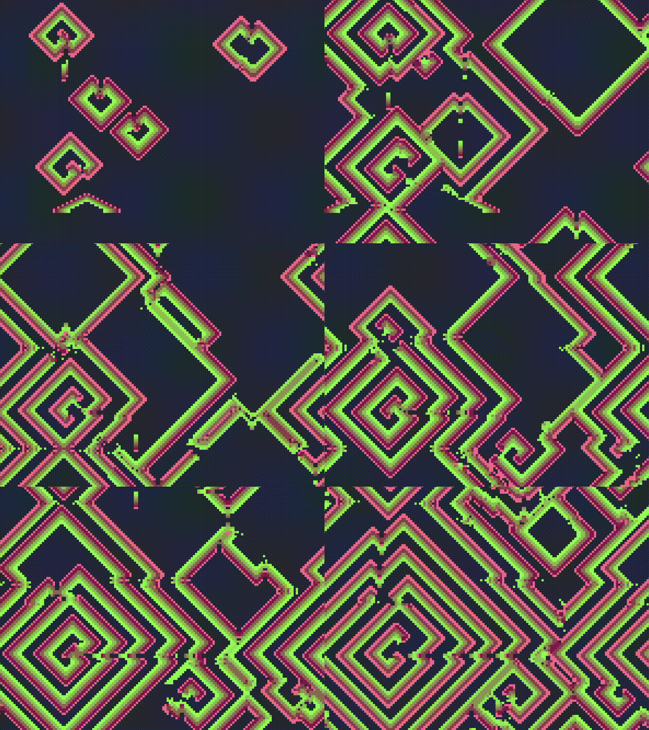
According to this generalization (let’s call it the NLUKY Rule), Life is NLUKY 03323 and Brain is NLUKY 12299. Walker discovered some other interesting rules which are shown below.

Cooties (NLUKY 72223)

Show

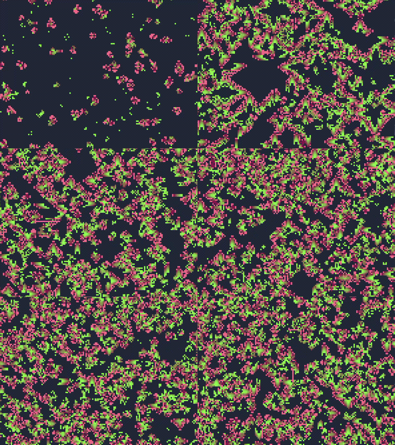
Faders (NLUKY 72222)

Show

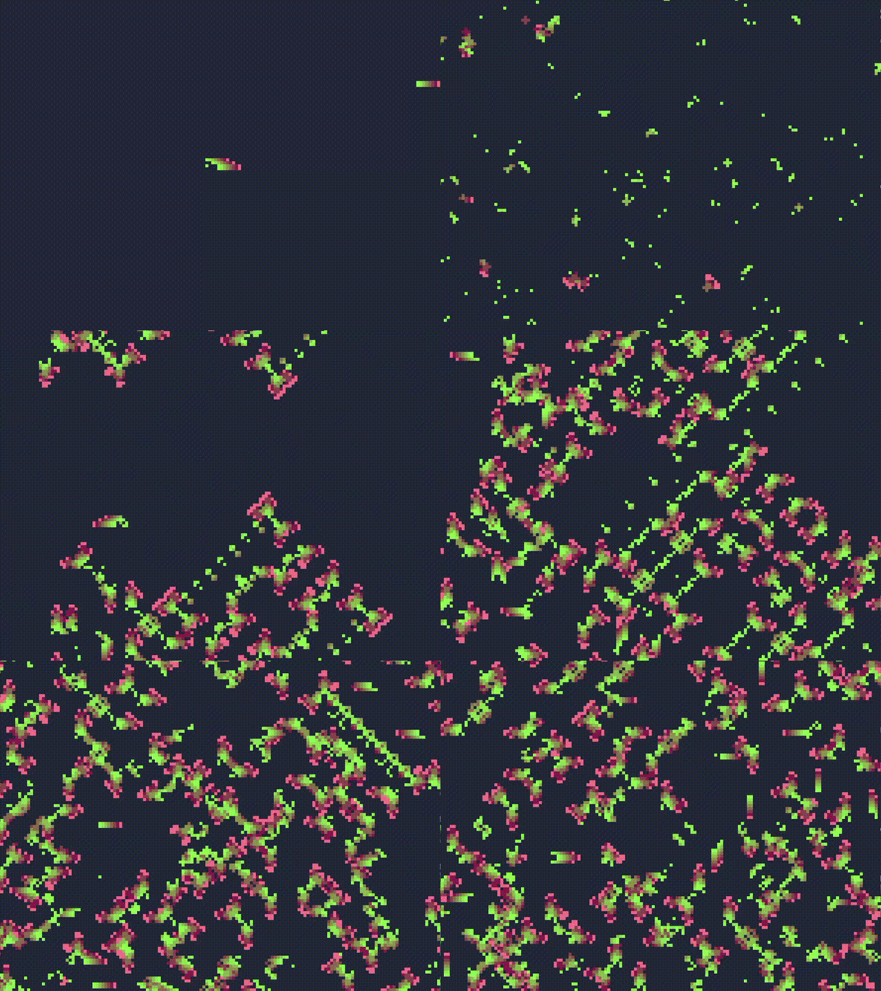
RainZha (NLUKY 72322)

Show

Elemenatry Cellular Automata (ECA)

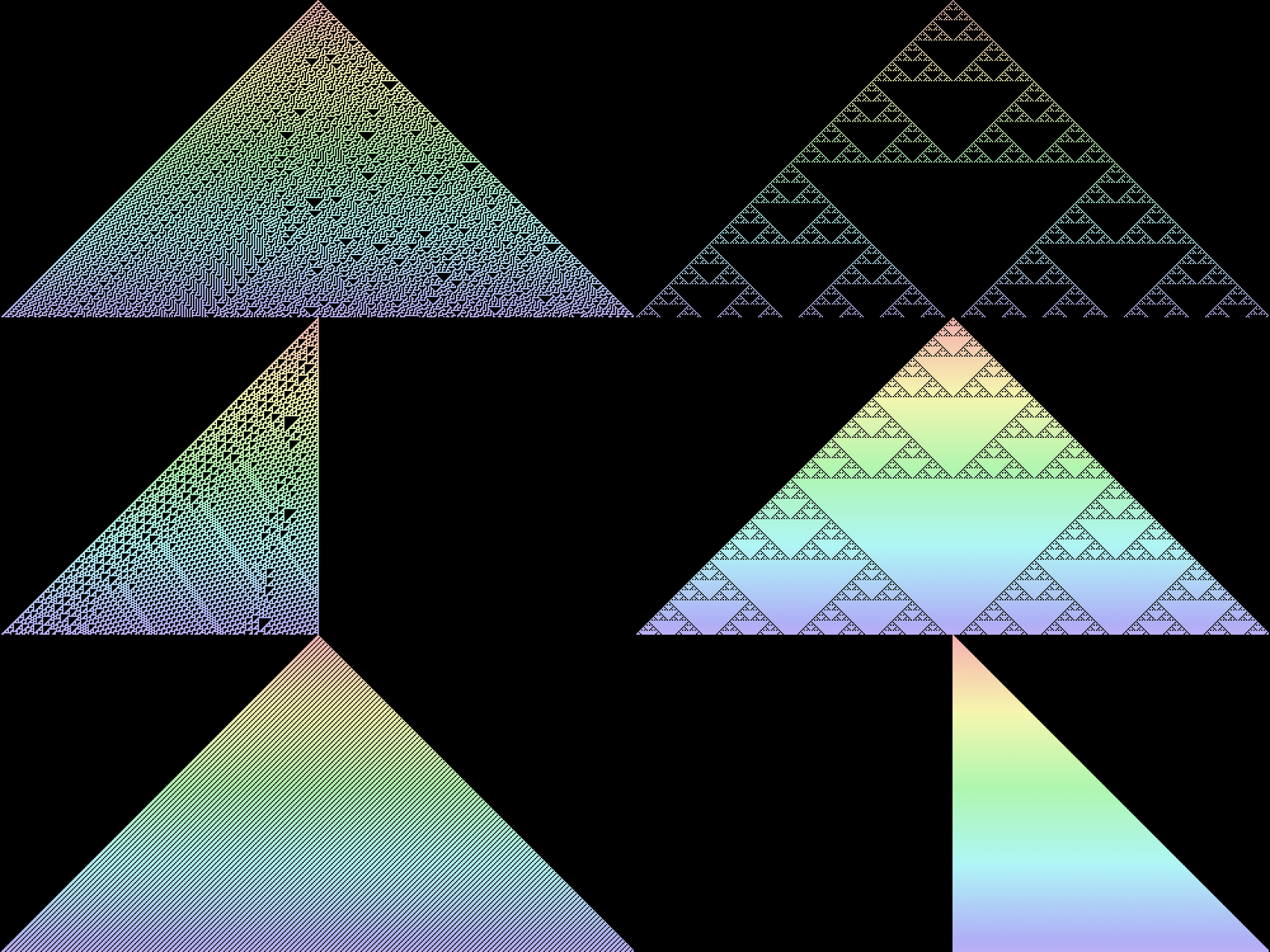
All the Celluar Automata I’ve discussed in this article up to this point have been two-dimensional. Let’s switch gears and look at one-dimensional Cellular Automata. ECA are the simplest form of one-dimensional Cellular Automata. Each cell has two possible states 0 or 1 and its state depends only on that of its two neareset neighbors and itself as shown in the figure below.